Window functions allow you to perform calculations against a subset of rows. The result of this calculation is shown against each row. This subset of rows in which you perform the calculation can be thought of as a window. This is achieved by using the SQL OVER clause. Within the OVER clause we can specify the subset of rows we wish to use. The function can then compute the value based upon the definition.
Microsoft have enhanced the implementation of window functions over time. In particular SQL Server 2012 when new window functions became available and the introduction of window frames.
Basic Syntax
The basic syntax is made up of the following:
-- Basic Syntax for the OVER clause
OVER (
       [ <PARTITION BY clause> ]
       [ <ORDER BY clause> ]
       [ <ROW or RANGE clause> ]
 )
- OVER – the clause where we define our windows function.
- PARTITION BY – determines how we divide the records up. The division of the records determines what subset of rows we perform our calculation on. You can perform the function without the partition clause; this will perform the calculation across all of the rows.
- ORDER BY – defines what order the rows will be processed within the window. This clause may or may not be optional depending on what type of window function is being performed.
- ROW or RANGE – allows us to define a FRAME within our framework, allowing further restriction of the subset of records processed for each row. For example it is possible to look at the previous 2 rows when performing our calculation rather than the full partition. ROWS or RANGE requires that the ORDER BY clause be specified. This implementation came in from SQL Server 2012. The difference between ROW and RANGE is explained later on in the post.
A simple example of window functions using one of the Stack Overflow sample databases is shown below. We will show for one user the total score for all their comments against each individual comment record.
USE StackOverflow2010;
GO

SELECT	UserId,
		Score,
		SUM(Score) OVER (PARTITION BY UserId) AS TotalUserScore

FROM	dbo.Comments

WHERE	UserId = 2515;
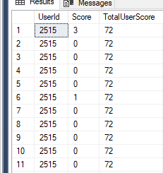
We use the PARTITION keyword to divide the rows by user. In this instance there is no need to include an ORDER by clause. Looking at the output we can see for each line we have the total user score.
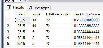
This technique allows us to easily work out what percentage a persons individual score makes up against their total, as shown below.
SELECT	UserId,
		Score,
		SUM(Score) OVER (PARTITION BY UserId) AS TotalUserScore,

		(Score * 1.0) / SUM(Score) OVER (PARTITION BY UserId) AS PercOfTotalScore

FROM	dbo.Comments

WHERE	UserId = 2515

ORDER	BY PercOfTotalScore DESC;
Without window functions we would need to write a subquery to the same table.
SELECT	c.UserId,
		c.Score,
		s.TotalScore,
		(Score * 1.0) / s.TotalScore AS PercOfTotalScore

FROM	dbo.Comments c

		INNER JOIN (

			SELECT	UserId,
					SUM(Score) AS TotalScore
			FROM	dbo.Comments
			GROUP	BY UserId

		) s ON c.UserId = s.UserId

WHERE	c.UserId = 2515
ORDER	BY  PercOfTotalScore DESC;
The window functions gives us a cleaner way of doing this.
Ranking Functions
Window functions can be grouped into three different types. Ranking functions will return a ranking value for each row in a partition. Depending on the function that is used, some rows might receive the same value as other rows while some may not.
There are four ranking functions we can use with window functions; ROW_NUMBER, RANK, DENSE_RANK and NTILE.
Let’s setup and show an example of how they work and differ between one another.
IF OBJECT_ID('tempdb..#TestAggregation') IS NOT NULL
	DROP TABLE #TestAggregation;
GO

CREATE TABLE #TestAggregation (

  SalesID		int				NOT NULL IDENTITY(1,1) PRIMARY KEY,
  SalesGroup	varchar(30)		NOT NULL,
  Country		varchar(30)		NOT NULL,
  AnnualSales	int				NOT NULL

);

GO

INSERT INTO #TestAggregation
  (SalesGroup, Country, AnnualSales)
VALUES
  ('North America', 'United States', 22000),
  ('North America', 'Canada', 32000),
  ('North America', 'Mexico', 28000),
  ('Europe', 'France', 19000),
  ('Europe', 'Germany', 22000),
  ('Europe', 'Italy', 18000),
  ('Europe', 'Greece', 16000),
  ('Europe', 'Spain', 16000),
  ('Europe', 'United Kingdom', 32000),
  ('Pacific', 'Australia', 18000),
  ('Pacific', 'China', 28000),
  ('Pacific', 'Singapore', 21000),
  ('Pacific', 'New Zealand', 18000),
  ('Pacific', 'Thailand', 17000),
  ('Pacific', 'Malaysia', 19000),
  ('Pacific', 'Japan', 22000);
GO
Using the test data we can run each of the functions together. Note we are running WITHOUT a PARTITION clause so the window will be across all of the available results.
SELECT	SalesGroup,
		Country,
		AnnualSales,
		ROW_NUMBER() OVER(ORDER BY AnnualSales DESC) AS RowNumber,
		RANK() OVER(ORDER BY AnnualSales DESC) AS BasicRank,
		DENSE_RANK() OVER(ORDER BY AnnualSales DESC) AS DenseRank,
		NTILE(3) OVER(ORDER BY AnnualSales DESC) AS NTileRank

FROM	#TestAggregation;
This results in the following output:
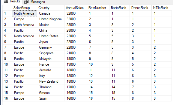
The ROW_NUMBER function simply numbers each row in the partition based upon the ORDER clause, which in this case is the column AnnualSales; highest to lowest. Because the statement returns 16 rows and there is only one partition, the rows are numbered 1 through 16.
The RANK function also numbers each row consecutively, based on the sorted AnnualSales values, but also takes into account duplicate values by assigning those values the same rank and then skipping the rank value that would have been assigned to the second duplicate. For example, the first 2 rows are ranked 1, so the third row is ranked 3 because the 2 has been skipped.
The DENSE_RANK function takes a slightly different approach. It accounts for duplicates but doesn’t skip ranking values. Consequently, the first 2 rows receive a ranking value of 1, as with RANK, but the third row receives a value of 2.
The NTILE function creates buckets / groups. If you refer back to the SELECT statement, you’ll notice that I passed a value of 3 in as an argument to the function.
As a result, the function divides the partition into 3 groups. That division is based on the total number of rows divided by the number specified in the function’s argument.
In this case, the 16 rows in the result set are divided into 1 group of six rows and 2 groups of five rows. The function assigns a 1 to each row in the first group, a 2 to each row in the second group, and a 3 to each row in the third group.
If we now add a PARTITION clause on the SalesGroup column to each of the statements we get the following:
SELECT	SalesGroup,
		Country,
		AnnualSales,
		ROW_NUMBER() OVER(PARTITION BY SalesGroup ORDER BY AnnualSales DESC) AS RowNumber,
		RANK() OVER(PARTITION BY SalesGroup ORDER BY AnnualSales DESC) AS BasicRank,
		DENSE_RANK() OVER(PARTITION BY SalesGroup ORDER BY AnnualSales DESC) AS DenseRank,
		NTILE(3) OVER(PARTITION BY SalesGroup ORDER BY AnnualSales DESC) AS NTileRank

FROM	#TestAggregation;
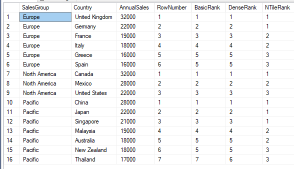
The functions work is the exact same way but gets reset between the partitions; the SalesGroup column in this case.
Analytical Functions
Coming in with the release of SQL Server 2012 these functions allow to you to include for each row, a value from another row. Two of the most used of these function are LAG and LEAD. LAG allows you to include a value from a previous row and LEAD allows you to include a value from an upcoming row. The sequence of these rows is dictated by the ORDER clause.
In the below example, for each row we will get the previous annual sales value and the upcoming annual sales value based upon annual sales being ordered from high to low. This will be partitioned by the SalesGroup which will reset the sequence when it changes.
SELECT	SalesGroup,
		Country,
		AnnualSales,
		LAG(AnnualSales, 1) OVER(PARTITION BY SalesGroup ORDER BY AnnualSales DESC) AS PreviousSale,
		LEAD(AnnualSales, 1) OVER(PARTITION BY SalesGroup ORDER BY AnnualSales DESC) AS NextSale

FROM	#TestAggregation

WHERE	SalesGroup IN ('Europe', 'North America')

ORDER	BY SalesGroup, AnnualSales DESC;
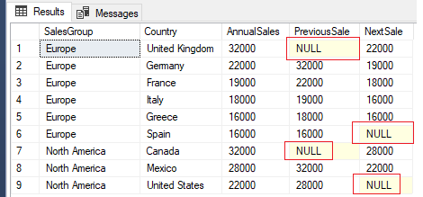
Row number 2 for Germany has the value of 32000 for the column PreviousSale which is the annual sales amount for United Kingdom, and 1900 for the NextSale column which is the annual sales amount for France.
For the first and last values in the sequence per SalesGroup category for LAG and LEAD respectively the values are NULL as no values exist.
The remaining two analytical functions FIRST_VALUE and LAST_VALUE allow you to return either the first row or last row from the defined partition.
Aggregation Functions
Aggregation functions allow you to perform one of the normal aggregation functions like COUNT or SUM but without the rows becoming grouped into a single output row. Aggregate functions don’t require an ORDER by clause, but from SQL Server 2012 can include one. If one is included then they can also use the ROWS or RANGE clause. If an ORDER BY is added and a ROWS/RANGE subclause is not defined then it will use the default options.
Let’s take a look at some examples using the same test data. We will calculate window functions for COUNT, SUM, and AVG.
SELECT	SalesGroup,
		Country,
		AnnualSales,
		COUNT(AnnualSales) OVER(PARTITION BY SalesGroup) AS CountryCount,
		SUM(AnnualSales) OVER(PARTITION BY SalesGroup) AS TotalSales,
		AVG(AnnualSales) OVER(PARTITION BY SalesGroup) AS AverageSales

FROM	#TestAggregation

WHERE	SalesGroup IN ('Europe', 'North America')
ORDER	BY SalesGroup, AnnualSales DESC;
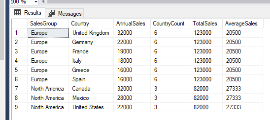
The columns CountryCount, TotalSales, and AverageSales all show the same result across all records which have the same SalesGroup, since it was the specified partition.
Let’s add an ORDER by clause into the code. but leave out the ROW or RANGE clause.
SELECT	SalesGroup,
		Country,
		AnnualSales,
		COUNT(AnnualSales) OVER(PARTITION BY SalesGroup ORDER BY AnnualSales DESC) AS CountryCount,
		SUM(AnnualSales) OVER(PARTITION BY SalesGroup ORDER BY AnnualSales DESC) AS TotalSales,
		AVG(AnnualSales) OVER(PARTITION BY SalesGroup ORDER BY AnnualSales DESC) AS AverageSales

FROM	#TestAggregation

WHERE	SalesGroup IN ('Europe', 'North America');
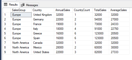
With the introduction of the ORDER BY clause we also bring into play the RANGE or ROW clause. As it was not specified it will use the default value. This is RANGE UNBOUNDED PRECEDING AND CURRENT ROW. This means that for each row in the partition, the window function is applied to the current row and all of the preceding rows. The upcoming rows are not taken into consideration. This means for each column we get the following results:
- CountryCount – rolling total counting the number of rows.
- TotalSales – rolling total based upon the ORDER clause. For example France is 73000 because it is made up of United Kingdom (32000) + Germany (22000) + France (19000).
- AverageSales – rolling average of the rows. For example Germany is 27000 because it is made up of United Kingdom and Germany, (3200 + 2200) / 2 = 2700.
The default window frame applies only to functions that have can accept optional ROWS/RANGE specification.
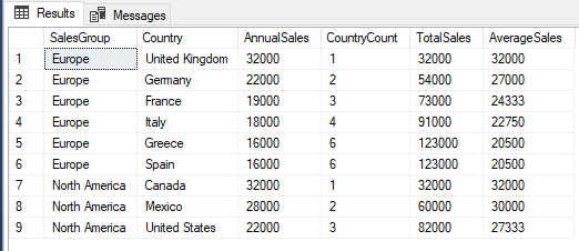
If we add in the window frame clause explicitly then we will get the same result.
SELECT	SalesGroup,
		Country,
		AnnualSales,
		COUNT(AnnualSales) OVER(PARTITION BY SalesGroup ORDER BY AnnualSales DESC RANGE BETWEEN UNBOUNDED PRECEDING AND CURRENT ROW) AS CountryCount,
		SUM(AnnualSales) OVER(PARTITION BY SalesGroup ORDER BY AnnualSales DESC RANGE BETWEEN UNBOUNDED PRECEDING AND CURRENT ROW) AS TotalSales,
		AVG(AnnualSales) OVER(PARTITION BY SalesGroup ORDER BY AnnualSales DESC RANGE BETWEEN UNBOUNDED PRECEDING AND CURRENT ROW) AS AverageSales

FROM	#TestAggregation

WHERE	SalesGroup IN ('Europe', 'North America');
Window Frames – Row vs Range
Looking at the previous results for Greece and Spain we see something interesting; they have the same results for CountryCount, TotalSales and AverageSales. This is because the RANGE option includes all rows which have the same ORDER BY value. Because the AnnualSales value, which is used in the ORDER by clause for Greece and Spain is 1600 the results get combined.
If we change the window frame to use ROWS instead of RANGE then each row is treated separately and we get a different result.
SELECT	SalesGroup,
		Country,
		AnnualSales,
		COUNT(AnnualSales) OVER(PARTITION BY SalesGroup ORDER BY AnnualSales DESC ROWS BETWEEN UNBOUNDED PRECEDING AND CURRENT ROW) AS CountryCount,
		SUM(AnnualSales) OVER(PARTITION BY SalesGroup ORDER BY AnnualSales DESC ROWS BETWEEN UNBOUNDED PRECEDING AND CURRENT ROW) AS TotalSales,
		AVG(AnnualSales) OVER(PARTITION BY SalesGroup ORDER BY AnnualSales DESC ROWS BETWEEN UNBOUNDED PRECEDING AND CURRENT ROW) AS AverageSales

FROM	#TestAggregation

WHERE	SalesGroup = 'Europe'

ORDER	BY SalesGroup, AnnualSales DESC;

Hopefully this post provides a good overview of window functions and how can then be implemented within SQL Server.