I have recently been working on a solution centred around reseller sales. We wanted to be able to analyse sales across several different entities such as product, vendor, delivery type and date. The source data comes from a single line of business system which can produce two unique files; a file with a list of products and a file containing sales data. Additional lookup data is stored in Microsoft Excel files. In this scenario there were no options for making use of a dedicated Datawarehouse or developing robust ETL pipelines from the source system. The solution needed to be as a simple as possible to minimise maintenance. We decided upon using Power BI to develop the solution and banked on using Power Query to transform and shape the data into an efficient model for data visualisations and analytics.
What is Power Query?
Power Query is a lightweight extract transform load (ETL) tool which is used in Power BI (as well as other Microsoft products). It allows for data transformation and data preparation to take place. Power Query provides users with the ability to model and shape data within Power BI before the datasets are used for report development and data visualisation. Power Query allows users to perform data preparation without the need for common enterprise options such as data pipelines tools like Azure Data Factory or SSIS, or dimensional designed data warehouses.
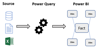
It can be used to create transformation pipelines at pace and was very useful in this scenario as it allowed us to keep the full end to end solution in a single tool. We wanted to use Power Query to transform our source files, made up of several flat files into a Dimensional Model.
What is a dimensional model?
Dimensional modelling (OLAP) is the process of modelling data into a structure which is optimised for data reporting. It is designed to read, aggregate and analyse numeric information in a highly efficient manner. This model is very different to your typical design used in line of business systems (OLTP); those models normalise data to reduce redundancy in the data. This allows for quick insert, update and delete operations. In contrast dimensional models don’t care for quick insert, update and delete operations so denormalise some data to improve read speeds.
A common dimensional model design pattern is the Star Schema invented by Ralph Kimball. This is where tables are split into two categories: dimensions and facts. A dimension table provides the context surrounding a process event. In our sales activity example this would be a table describing a product, or a table describing the dates an order was made. Dimension tables are used to slice and dice the numerical data held within the fact. A fact table holds the numerical information from the business process event at a specific granularity. In our sales activity example, we store one row per order line processed. Examples of measures stored against each row would include the price paid by a customer, the quantity of items ordered, and the profit made from the transaction. These measures are aggregated up and analysed by attributes within the dimension. Dimensions are connected to facts directly across a single join. Multiple facts tables can be connected through shared dimensions, known as conformed dimensions.
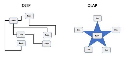
Power BI has been optimised for performance against a star schema model so made perfect sense to implement the model.
Implementing in Power Query
We used Power Query to transform our flat file data source files into a star schema model. Here is an illustration of the design at the start and what it looked like at the end.

Power Query transforms queries with steps. Each step is a different transformation done on the data. This is a useful approach as you can visualise the change in the data through each step by clicking on it. You can also add in steps in the middle of the process / remove a certain step if it needs tweaking. It does also sometimes make working in Power Query quite slow as it processes all of the steps in memory.
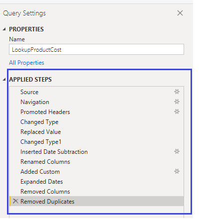
We will discuss some of the main parts we work through to create this model.
Dynamic file names and location
The first step to start the process was to import the base files into Power Query. We made use of the multiple data connectors Power Query has available to do this via the new source menu.
- Sales data can come in multiple files which all have the same format. We connected to this data using the folder connector. This allowed us to import and merge multiple files into a single query.
- The lookup files are stored in Microsoft Excel so we used the Excel connector to import these.
- The product file is stored in a csv so we used the Text/Csv connector to import this file.
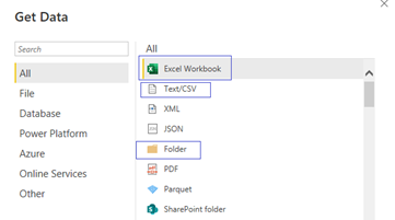
When the connections are setup in Power Query the connection string will hard code the folder path to the files.

To improve maintainability we made use of parameters to hold the names of files, folders, and folder paths. This is useful, particularly with text and Excel files where we may change around the folder structure or move the full setup to another computer which has a completely different folder structure. In this case we setup parameters to hold the folder path, subfolder, and file names.
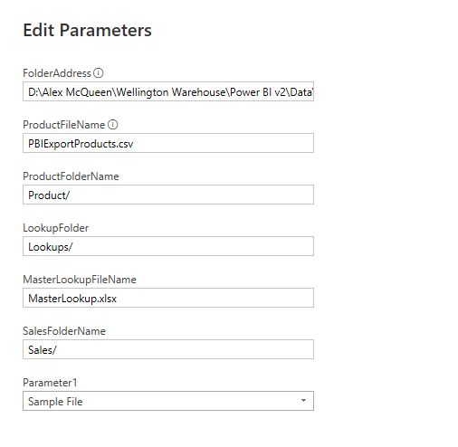
We incorporated these variables into the connection string. If the paths need to be changed in the future we can just updated the parameters.

Creating a dimension from the sales file
Some of the dimensions we needed to create did not have their own data source; they needed to be created from the sale files. We made use of the reference feature in Power Query for this. Reference is a way of copying a query. When you reference you just reference the original query rather than making a physical copy of it. We used this technique to create the fact and some of the dimension tables.
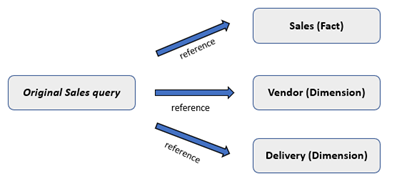
The creation of the dimension tables followed the same pattern shown below.
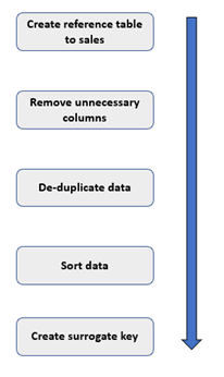
Once we had created the reference to the sales query we removed all the columns we didn’t need.
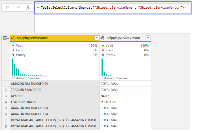
We then removed the duplicates from the remaining columns giving us a unique list. At this stage we ordered the list. This ensured the index we created after is always in the same order.
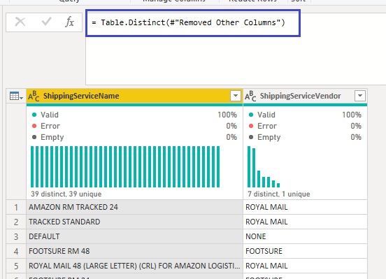
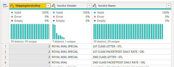
We created an index column incrementing from 1, renamed and reordered the columns. This left us with the delivery dimension looking like the below.
Dealing with slowly changing attributes
The business needs to maintain several lookup Microsoft Excel sheets to hold information about costs that change over time. For example, when an order is delivered to a customer, it will be done by a specific company who will charge a fee. However, this rate can change over time and that change is not captured in the line of business system. To account for this the business holds the changes in an Excel spreadsheet. For each delivery business and delivery type a cost will be held with a start and end date. When the cost changes a new line is input and the dates are amended accordingly. This date needs to be applied against the sales to determine the cost based upon when the sale took place.

This file in it’s current format presented a problem for Power Query. We wanted to merge this file with the sales file but did not have an equality join. We would want to join using a range of dates; for example matching the delivery type but then checking the sales date falls into between the start and end date. However this is difficult in Power Query.
One way to solve this is to convert the data granularity of the lookup table to have one row per date for each date between the start and end dates of each row. This would then allow for an equality join to take place. Below is the pattern I used:
- Convert the default end date to an earlier date. This reduces the number of rows we are going to generate.
- Calculate the duration between the start and end dates. This gives the number of rows we needed to generate for each record.
- Create a list of dates, going from the start date and incrementing up a day for the duration number.
- Expand the list to show the dates.

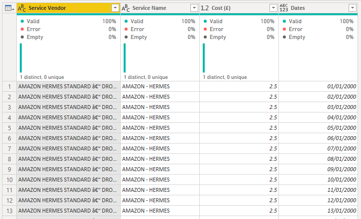
- Use these dates to connect the table to the sales table using the received date and place on the correct cost.
Once the query had been transformed we were easily able to connect it to the sale table and merge over the correct costs.
Connecting dimensions to facts
Once we had created all of the dimensions we needed to link them to the fact. This again followed a specific pattern for all of the dimensions.
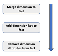
The sale table at this stage had all of the original columns. We used these to create a unique join between the sales table and each dimension like the below shows.
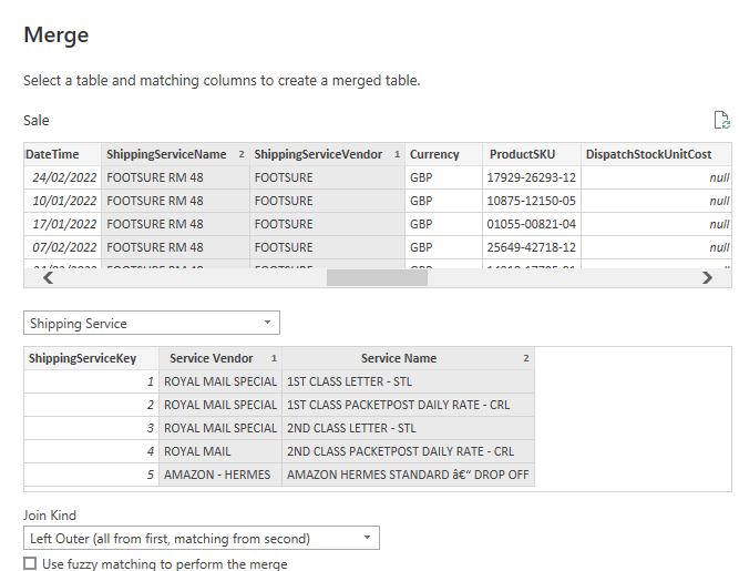
Once we had merged the tables and brought over the index key we made when creating the dimensions, we could discard the dimension attributes in the original sale table. This would leave us with the numeric columns and dimension keys in the sale table.
Final Model
The transformations performed in Power Query allowed us to create the dimensional model shown below. This model would result in easier report design and development.
